| 일 | 월 | 화 | 수 | 목 | 금 | 토 |
|---|---|---|---|---|---|---|
| 1 | 2 | 3 | ||||
| 4 | 5 | 6 | 7 | 8 | 9 | 10 |
| 11 | 12 | 13 | 14 | 15 | 16 | 17 |
| 18 | 19 | 20 | 21 | 22 | 23 | 24 |
| 25 | 26 | 27 | 28 | 29 | 30 | 31 |
- coursera
- andrew ng
- AI
- Python
- localization
- docker
- internationalization
- deeplearning.ai
- gettext
- gettext_windows
- 국제화
- I18N
- 현지화
- Today
- Total
JMANI
Ray Tune Documentation 본문
ref: https://docs.ray.io/en/latest/tune/index.html
Tune: Scalable Hyperparameter Tuning — Ray 1.13.0
Learn how to use Ray Tune for various machine learning frameworks in just a few steps. Click on the tabs to see code examples. Tip We’d love to hear your feedback on using Tune - get in touch! To run this example, install the following: pip install "ray[
docs.ray.io
import numpy as np
import torch
import torch.optim as optim
import torch.nn as nn
from torchvision import datasets, transforms
from torch.utils.data import DataLoader
import torch.nn.functional as F
import matplotlib.pyplot as plt
import os
from ray import tune
from ray.tune.schedulers import ASHAScheduler
from hyperopt import hp
from ray.tune.suggest.hyperopt import HyperOptSearch
# Change these values if you want the training to run quicker or slower.
EPOCH_SIZE = 512
TEST_SIZE = 256
class ConvNet(nn.Module):
def __init__(self):
super(ConvNet, self).__init__()
# In this example, we don't change the model architecture
# due to simplicity.
self.conv1 = nn.Conv2d(1, 3, kernel_size=3)
self.fc = nn.Linear(192, 10)
def forward(self, x):
x = F.relu(F.max_pool2d(self.conv1(x), 3))
x = x.view(-1, 192)
x = self.fc(x)
return F.log_softmax(x, dim=1)
def train(model, optimizer, train_loader):
device = torch.device("cuda" if torch.cuda.is_available() else "cpu")
model.train()
for batch_idx, (data, target) in enumerate(train_loader):
# We set this just for the example to run quickly.
if batch_idx * len(data) > EPOCH_SIZE:
return
data, target = data.to(device), target.to(device)
optimizer.zero_grad()
output = model(data)
loss = F.nll_loss(output, target)
loss.backward()
optimizer.step()
def test(model, data_loader):
device = torch.device("cuda" if torch.cuda.is_available() else "cpu")
model.eval()
correct = 0
total = 0
with torch.no_grad():
for batch_idx, (data, target) in enumerate(data_loader):
# We set this just for the example to run quickly.
if batch_idx * len(data) > TEST_SIZE:
break
data, target = data.to(device), target.to(device)
outputs = model(data)
_, predicted = torch.max(outputs.data, 1)
total += target.size(0)
correct += (predicted == target).sum().item()
return correct / total
def train_mnist(config):
# Data Setup
mnist_transforms = transforms.Compose(
[transforms.ToTensor(),
transforms.Normalize((0.1307, ), (0.3081, ))])
train_loader = DataLoader(
datasets.MNIST("~/data", train=True, download=True, transform=mnist_transforms),
batch_size=64,
shuffle=True)
test_loader = DataLoader(
datasets.MNIST("~/data", train=False, transform=mnist_transforms),
batch_size=64,
shuffle=True)
device = torch.device("cuda" if torch.cuda.is_available() else "cpu")
model = ConvNet()
model.to(device)
optimizer = optim.SGD(
model.parameters(), lr=config["lr"], momentum=config["momentum"])
for i in range(10):
train(model, optimizer, train_loader)
acc = test(model, test_loader)
# Send the current training result back to Tune
tune.report(mean_accuracy=acc)
if i % 5 == 0:
# This saves the model to the trial directory
torch.save(model.state_dict(), "./model.pth")
# Uncomment this to enable distributed execution
# `ray.init(address="auto")`
"""
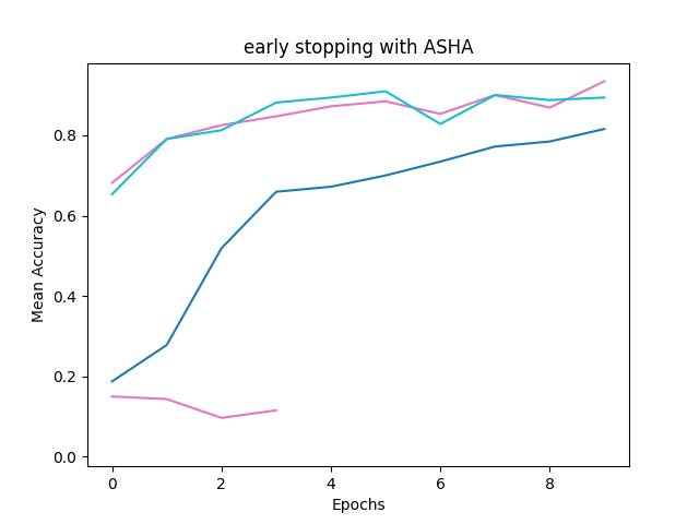
Early Stopping with ASHA
search space increasing > parameter <num_samples>
ASHA is implemented in Tune as a “Trial Scheduler”.
These Trial Schedulers can early terminate bad trials,
pause trials, clone trials,
and alter hyperparameters of a running trial.
"""
def ASHA_scheduler(search_space):
scheduler = \
ASHAScheduler(metric="mean_accuracy", mode="max")
# Obtain a trial dataframe from all run trials of this `tune.run` call.
ASHA_anno = "early stopping with ASHA"
# num_samples: grid search 반복 횟수 default:1
analysis = tune.run(
train_mnist,
num_samples=20,
scheduler=scheduler,
config=search_space,
)
dfs = analysis.trial_dataframes
plot(dfs, ASHA_anno)
bt_model = best_model(analysis)
return bt_model
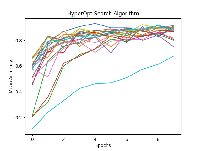
def HyperOpt_search_alg(space):
search_alg = \
HyperOptSearch(space, metric="mean_accuracy", mode="max")
# Obtain a trial dataframe from all run trials of this `tune.run` call.
HyperOpt_anno = "HyperOpt Search Algorithm"
analysis = tune.run(train_mnist,
num_samples=20,
search_alg=search_alg)
# To enable GPUs, use this instead:
# analysis = tune.run(
# train_mnist, config=search_space, resources_per_trial={'gpu': 1})
dfs = analysis.trial_dataframes
plot(dfs, HyperOpt_anno)
bt_model = best_model(analysis)
return bt_model
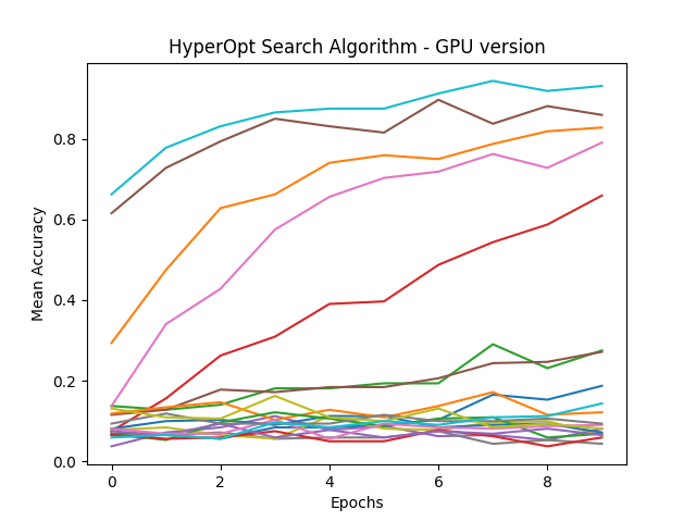
def gpu_HyperOpt_search_alg(space):
# Obtain a trial dataframe from all run trials of this `tune.run` call.
HyperOpt_anno = "HyperOpt Search Algorithm - GPU version"
analysis = tune.run(train_mnist,
config=space,
num_samples=20,
resources_per_trial={'cpu': 2, 'gpu': 1})
# To enable GPUs, use this instead:
# analysis = tune.run(
# train_mnist, , resources_per_trial={'gpu': 1})
dfs = analysis.trial_dataframes
plot(dfs, HyperOpt_anno)
bt_model = best_model(analysis)
return bt_model
def plot(dfs, name):
# Plot by epoch
ax = None # This plots everything on the same plot
for d in dfs.values():
ax = d.mean_accuracy.plot(ax=ax, legend=False)
ax.set_xlabel("Epochs")
ax.set_ylabel("Mean Accuracy")
plt.title(name)
plt.savefig(os.path.join('img', name + '.jpg'))
plt.show()
def best_model(analysis):
df = analysis.results_df
print(df)
logdir = analysis.get_best_logdir("mean_accuracy", mode="max")
state_dict = torch.load(os.path.join(logdir, "model.pth"))
model = ConvNet()
model.load_state_dict(state_dict)
return model
if __name__ == "__main__":
a = tune.sample_from(lambda spec: 10 ** (-10 * np.random.rand()))
search_space = {
"lr": tune.sample_from(lambda spec: 10 ** (-10 * np.random.rand())),
"momentum": tune.uniform(0.1, 0.9),
}
space = {
"lr": hp.uniform("lr", 1e-10, 0.1),
"momentum": hp.uniform("momentum", 0.1, 0.9),
}
# TrialScheduler
ASHA_scheduler(search_space)
# Search Algorithm
HyperOpt_search_alg(space)
# GPU Search Algorithm
# 속도가 오래걸리는 이유: 1 trials 당 gpu 1개를 할당하기 때문
gpu_HyperOpt_search_alg(search_space)
- num_samples
search space를 num배 만큼 증가시킬 수 있다. 아래 예에서 3X3 grid_search를 num_samples(10)번 반복하기 때문에 총 90번의 시도(검색)를 하게 된다.
ref: https://docs.ray.io/en/latest/tune/tutorials/tune-search-spaces.html
 tune.run(
     my_trainable,
     name="my_trainable",
     # num_samples will repeat the entire config 10 times.
     num_samples=10
     config={
         # ``sample_from`` creates a generator to call the lambda once per trial.
         "alpha": tune.sample_from(lambda spec: np.random.uniform(100)),
         # ``sample_from`` also supports "conditional search spaces"
         "beta": tune.sample_from(lambda spec: spec.config.alpha * np.random.normal()),
         "nn_layers": [

             # tune.grid_search will make it so that all values are evaluated.

             tune.grid_search([16, 64, 256]),
             tune.grid_search([16, 64, 256]),
         ],
     },
 )
- GPU 사용 및 자원 할당
gpu 사용을 위해 tune.run()의 resources_per_trial 파라미터를 설정한다. 1 시도 당 자원을 얼마나 할당할지 정하는 파라미터이다. 만약 내가 24개의 CPU, 2개의 GPU를 사용할 수 있다면, {'cpu': 2, 'gpu': 1}은 3개씩 시도할 수 있다.
GPU를 사용하기 때문에 속도가 더 빨라질 것을 예상했는데, gpu 사용이 훨씬, 몇배 느리다.
auto mode에서는 한번에 20개 이상의 cpu로 작업하지만, 자원을 설정해버리면 정해논 개수만큼만 사용하기 때문이다. 즉, 다른 작업이 끝날때까지 기다린다.
# auto
analysis = tune.run(train_mnist,
                    num_samples=20,
                    search_alg=search_alg)
# GPU
analysis = tune.run(train_mnist,
                        config=space,
                        num_samples=20,
                        resources_per_trial={'cpu': 2, 'gpu': 1})
또한, GPU 사용을 위해 search_space에 tune.sample_from(함수 호출 형태)로 바꿔줘야 한다.(docs에 나와있지만 이유는 모름)
search_space = {
    "lr": tune.sample_from(lambda spec: 10 ** (-10 * np.random.rand())),
    "momentum": tune.uniform(0.1, 0.9),
}